Numerical tools are used to obtain objective information from models. These are called targeting techniques.
One commonly distinguishes between two families and two generations of such techniques.

Two generations :

The two generations differ in the ability to account for the future observations to be routinely deploy in addition to the atmospheric dynamics.
Thus, the first-generation techniques give information on where changes, even small, in the initial modeled conditions (analysis) will have the greatest impact on the forecast in the verification domain.
The second-generation techniques give estimates of the expected reduction of the variance of the forecast error in the verification domain when considering simulated alternative deployments of supplementary observations. It can also give a less sharp information in the shape of maps showing the need for additional observation for a better prediction of the phenomenon to verify.

The adjoint-based family.

The technology uses the adjoint of the tangent linear version of the nonlinear prediction model (for both 1^st and 2^nd generations) and an estimate of the adjoint of assimilation system (for the 2^nd generation only).
Among this family, one can find the following techniques : the forecast sensitivity to its initial conditions (1), the total energy singular vectors (1), the Hessian singular vectors (2), the HRRE   (Hessian Reduced Rank Estimate, 2) and the KFS   (Kalman Filter Sensitivity, 2).

The ensemble-based family.

The techniques of this family use the properties of ensembles of forecasts to estimate variance and covariances of analysis and forecast errors. Moreover, with not too large ensembles one can define subspace in which it is convenient to compute the reduction of variance due to the addition of simulated observations. Excluding thecomputing cost of the ensemble itself, these techniques are generally less expensive than the adjoint-based techniques.
The most common technique is the ETKF   (Ensemble Transform Kalman Filter, 2).

Challenges :

The most advanced techniques take account for the atmospheric dynamics, the future observations, the data assimilation algorithms and for the uncertainty in the forecasts. These lie at the frontiers of current expertise in numerical weather prediction (NWP  ). Moreover, these techniques have to predict the coverage of the expected routine observations at the additional observations’ deployment time. The location and uncertainty (and error correlations) of these observations are the primary aspects to predict. But for much of the observations currently assimilated in NWP   models, such an observation location may depend on poorly predictable phenomena : position of the clouds (infrared satellite data, cloud motion-derived wind vectors), or choice of the aerial routes (data from commercial aircraft).

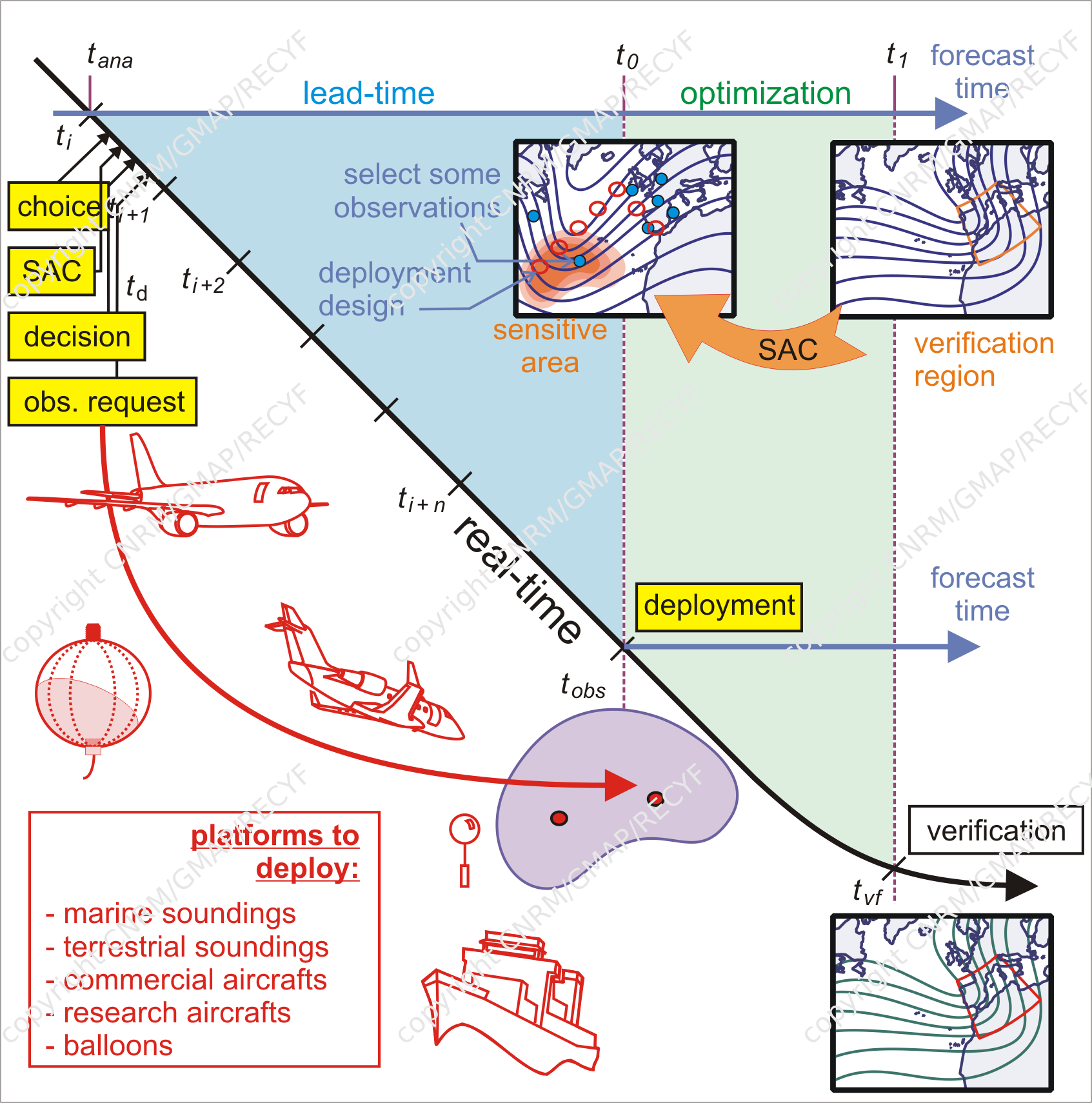
The issue of predicting the observational network also arises for the whole interval of time between now (daily calculations and decision making, t_ana in the diagram about principles) and the future time of deployment of the additional observations (t_obs). All the information these observations will introduce in the PNT   system before the deployment of targeted observation is currently ignored in the techniques.

Our techniques

In CNRM   (Météo-France), several techniques are either available or under development :

The sensitivity to initial conditions

The KFS

The ETKF

Example of sensitive area computed with the KFS  .

Sensitive area computed with the KFS

The purple shaded area shows the sensitive area (need for additional observations) computed with the KFS method on the case 1085 of the DTS-MEDEX experiment. Contours show the Z500 valid at targeting time. Dots and circles show the radiosounding sites (see legend above the map).

The purple shaded area shows the sensitive area (need for additional observations) computed with the KFS   method on the case 1085 of the DTS  -MEDEX   experiment. Contours show the Z500 valid at targeting time (t_obs). The orange square shows the verification region which is valid 18h later than targeting time. Dots and circles show the radiosounding sites (see legend above the map).

Example of sensitive area computed with the classical adjoint-based sensitivity.

Adjoint-based sensitivity

The greenish shaded area shows the sensitive area computed with the classical method called "sensitivity of the forecast to its initial conditions" on the case 1085 of the DTS-MEDEX experiment.

The greenish shaded area shows the sensitive area computed with the classical method called "sensitivity of the forecast to its initial conditions" on the case 1085 of the DTS  -MEDEX   experiment.The orange square shows the verification region which is valid 18h later than targeting time.

Example of composite targeting guidance computed with the ETKF  .

Composite trageting guidance computed with ETKF

The violet shadings show the composite fields generated by the ETKF method. The case is 1085 as well. Each grid point is rated with expected forecast error variance reduction due to the deployment of an observing probe in that point. Contours show the Z500 valid at targeting time. Dots and circles show the radiosounding sites (see legend above the map).

The violet shadings show the composite fields generated by the ETKF   method. The case is 1085 as well. Each grid point is rated with expected forecast error variance reduction due to the deployment of an observing probe in that point. Contours show the Z500 valid at targeting time (t_obs). The orange square shows the verification region which is valid 18h later than targeting time. Dots and circles show the radiosounding sites (see legend above the map).

References :

Bishop C.H., B. J. Etherton and S.J. Majumdar, 2001. Adaptive sampling with the ensemble transform Kalman filter. Part I : theoretical aspects. Monthly Weather Review, 129, 420—436.

Majumdar S.J., C.H. Bishop, B.J. Etherton and Z. Toth, 2001. Adaptive sampling with the Ensemble Transform Kalman Filter. Part II : Field program implementation. Monthly Weather Review, 130, 1356—1369.

Leutbecher M., 2003. A reduced rank estimate of forecast error changes due to intermittent modifications of the observing network. Journal of Atmospheric Sciences, 60 (5), 729—742.