3. Vincent GUIDARD : "Evaluation of assimilation cycles in a mesoscale limited area model"
Due to biperiodisation and to the length-scales of the
structure functions, some problems may occur when using observations near the
border of the C+I domain (cf. previous Newsletter).
Let ENIL1 and ENIL2 be the distance for starting the
modification of the covariances and the distance of effective zeroing,
respectively.
Let mask be the mask defined by :
To obtain compactly-supported ("COSU") autocorrelations, one has to
apply this mask in the gridpoint space :
qcosu (x, y) = q (x, y)
× mask( sqrt (x 2+
y 2) ),
which is the exact formula if the observation is located at (0,0). This
multiplication corresponds to a convolution in the spectral space :
F(qcosu)(m, n) = (
F(q)*F(mask))(m, n).
According to Gaspari and Cohn (1999), this mask should be applied to the
square root of the gridpoint correlations.
Therefore, the autocorrelations won't be exactly zero from ENIL2, but from
some distance between ENIL2 and 2x
ENIL2.
Here is the method used in this study, which has been proposed by Loïk
Berre :
The 1D model used in this study is a gridpoint model, with
289 gridpoints in the C+I domain and a 11-gridpoints wide E-zone, only used to
perform an analysis.
It is a univariable (so univariate) model. Everything is done in gridpoint
space. The formula used for the analysis is :
The 1D model provides an opportunity to evaluate the impact
of an enhancement of the length of the extension zone. In order to mimic such
a modification, with constant C+I zone, we have only to modify the horizontal
autocorrelations. It has been decided to extrapolate the missing values from
the original gridpoint variances. The extrapolated values are all equal to
each other and are continuous with the original values.
Figure 1 shows that there is no modification in the
neighbourhood of the observations. But the value of the analysis (and the
value of the analysis increment) at the border of C+I and E-zones is not the
same. The analysis increment at the border can be reduced to 22.5 % of its
initial value when using a three times bigger E-zone. Even if it was quite
obvious, this is a really positive cure to the "wrap-around'' effect due
to the biperiodisation.
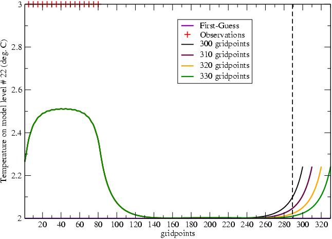
Figure 1: Observations, first-guess and analysis for various lengths of the
E-zone, for temperature on model level # 22.
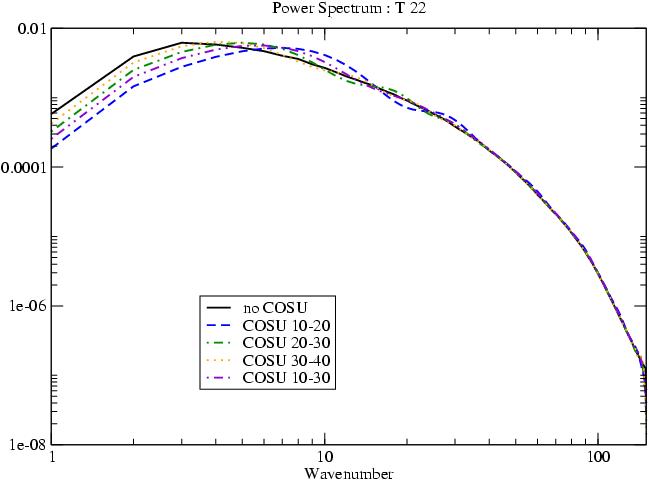
From now, "no COSU" refers to the original power
spectrum, and "COSU xx-yy" refers to compactly-supported
autocorrelations with ENIL1 =xx and ENIL2=yy (xx and
yy are gridpoint values; remember that ENIL2 is the distance of zeroing for
the square root of the autocorrelations).
The modified power spectra are obtained following the above-mentioned method.
The impact on the power spectrum, for various values of ENIL1 and ENIL2 (and
various combinations), is shown on Figure 2a. In a
global overview, since the autocorrelations are compactly supported, the
values of the power spectrum for the 3 first total wavenumbers are decreased.
There is hardly no change of the power spectrum for total wavenumbers ranging
from 40 to 140. Some oscillations appear when ENIL1 and ENIL2 -
ENIL1 are too small. The tuning "COSU 10-20" is to be
rejected, for instance.
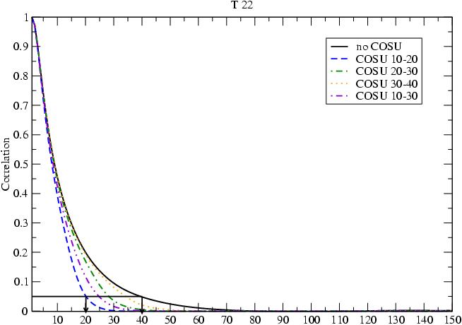
To observe the real impact on the autocorrelations in gridpoint space, the
power spectra previously generated are converted into gridpoint structures.
Figure 2b shows these gridpoint structures for the
reference ("no COSU") and various tunings of compact support. First,
with a zoom (not shown), one could notice that compactly-supported
autocorrelations are not exactly zero. It is due to not totally symmetric
steps (direct and inverse Fourier transforms, and fill-in of the ellipse and
collect). But the values for the COSU autocorrelations are quite satisfying :
for a distance greater than 50 gridpoints, values are less than 2.10-4
, that is to say less than 1/5000th of the maximum value. The
general impact is as expected.
|
Figure 2a: COSU power spectra for temperature on model level # 22. |
Figure 2b: COSU gridpoint autocorrelations for temperature on model level # 22. |
The decrease of the length-scale obtained for the gridpoint autocorrelations
is confirmed in the analysis of 15 observations (cf. Figure
3). The shape of the analysis increment is slightly modified. The values
of the analysis increment in the area containing no observations, and far
enough from the observations, are efficiently reduced thanks to the compact
support. This method also offers a cure to the "wrap-around" effect.
The value of the analysis increment at the border between C+I and E zones is
4.5 times smaller in the COSU experiment than in the reference (which is
equivalent to the results obtained with the modification of the E-zone length).
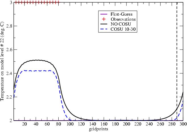
Figure 3: Observations, first-guess and analysis for COSU and non COSU
covariances, for temperature on model level # 22.
Following both the implementation of compactly-supported
horizontal correlations in ARPEGE (cf. routine SUJBCOSU
written by François Bouttier) and the first results of COSU horizontal
autocorrelations, the SUEJBCOSU routine has been
implemented in ALADIN, with the great help of Claude Fischer. Its purpose is
to compactly support the horizontal correlations and the vertical
cross-correlations (and also the horizontal balance).
The univariate case is the closest to what was done in the 1D model. The compact support has only to be applied to horizontal autocorrelations. COSU horizontal autocorrelations imply a damping of residual noise farther than a given distance (between ENIL2 and 2x ENIL2). Some geometric noise still remains (cross centered on the observation, plus a rhombus). But the results are quite the same as in the 1D model and encourage us to run a multivariate 3D-VAR with COSU horizontal autocorrelations.
The multivariate formulation used in this study is based on
the work of Loïk Berre (2000). In this section, single observation (of
temperature at 500 hPa) experiments are performed and compared through their
temperature analysis increment on model level # 15.
In this paragraph, only the horizontal autocorrelations are
compactly supported. Neither vertical cross-correlations nor balance operators
are modified. Some astonishing results are obtained. Though quite few benefits
(even neutral results) were expected, "worse" patterns are
generated. These results remain unchanged whatever the values of ENIL1 and
ENIL2. An explanation could be that the main part of the temperature increment
is balanced, while only the vorticity (z)
horizontal correlations are compactly supported, but not Hb
z, where Hb is the horizontal balance operator.
If we consider that the statistical inverse Laplacian H
b and the analytical inverse Laplacian D
-1 are
equivalent, Hbz is equivalent to
D -1z, that is to
say the streamfunction. The power spectrum of the vorticity can be modified to
obtain COSU horizontal correlations for the streamfunction. Compactly
supporting the streamfunction gives neutral results, but it allows to
eliminate the "worse and weird" increments. Moreover, using COSU
vertical cross-correlations additionally leads to the same results (that is a
mostly neutral impact).
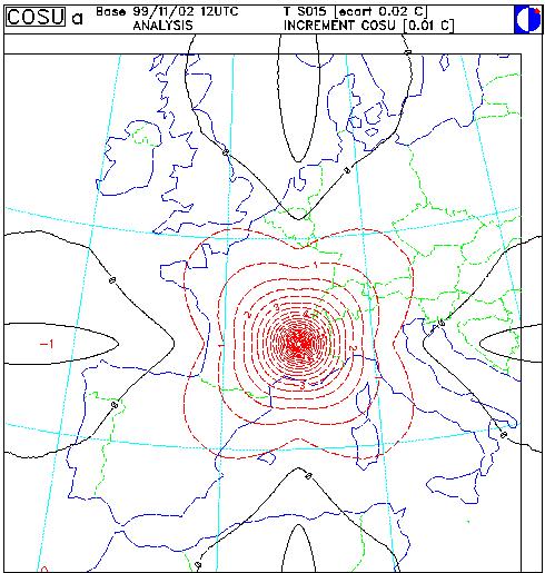
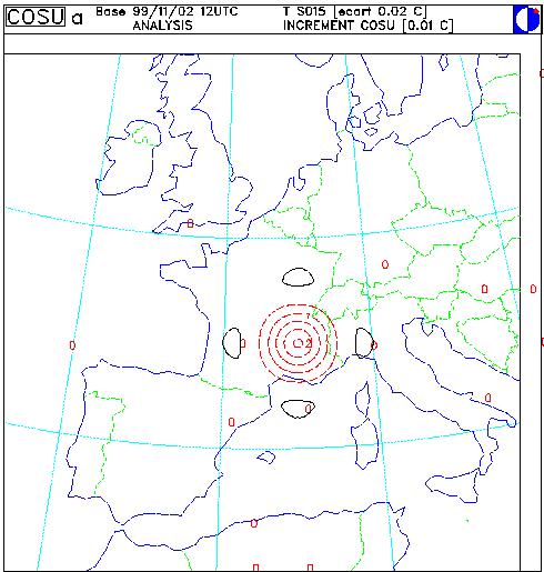
Another point of view, a bit more drastic, is to consider the
horizontal balance as an operator which can be compactly supported. The
compact support is first applied with "short" ENIL1 and ENIL2 (
Figure 4b, to be compared to the reference, Figure
4a). This method is really efficient in controlling the length-scale of
the increment. Note that COSU horizontal balance is an "antidote" to
COSU vorticity horizontal correlations. Other values for ENIL1 and ENIL2 have
been tested (not shown). It seems that the length-scale of the horizontal
balance is the leading one, as the shape of the increment seems to depend only
on what is applied to the horizontal balance. Some experiments using different
distances of zeroing for correlations and horizontal balance have been
performed. They reinforce the feeling that the horizontal balance is the most
important element to be modified to obtain COSU analysis increments.
|
Figure 4a: reference, with original B. |
Figure 4b: all COSU 10-30 (horizontal correlations, horizontal balance operator) |
All these single-observation experiments are only a step
towards the use of the SUEJBCOSU routine with real
observations on real cases. That is why preliminary tests of
compactly-supported structure functions are performed (not shown). First, a
band of observations (all observation types) over a southern third of the
domain is considered. There are only few changes in comparison to the
reference, but the "wrap-around" effect is a bit reduced.
As a second step, a 3D-VAR analysis is performed with all observations (i.e.
as "usual"). There is no modification, despite very short
distances of zeroing. This has to be further investigated.
Having a wide enough E-zone is important if all observations
inside the C+I domain are used : it prevents the analysis increment from
"wrapping around". But, one should be aware of the over-costs
generated by a drastic enhancement of the E-zone. In the case of ALADIN with a
289-gridpoints wide square C+I domain, a 320-gridpoints (or more) wide square
C+I+E domain is recommended.
To control the length-scale of the increment, compactly-supported horizontal
correlations can be used (background statistics). In the univariate case, this
is sufficient to have a real control. But in the multivariate case, it appears
that, to obtain similar results, the horizontal balance operator has to be
compactly supported too. As the distance of zeroing is tunable, one can
experiment different values to reach a "realistic" limit. To keep in
mind the theoretical benefit of COSU structure functions : for temperature on
model level # 22, the distance from which the horizontal correlation is less
than 0.05 is 400 km for the original B and only 250 km for the COSU
10-30 experiment.
Berre, L. (2000).
Estimation of synoptic and mesoscale forecast error covariances in a
limited-area model.
Mon. Wea. Rev. 128, 644-667.
Gaspari, G. and S. Cohn (1999).
Construction of correlation functions in two and three dimensions.
Quart. J. Roy. Meteor. Soc. 125 , 723-757.