Application of the Predictor-Corrector method to
non-hydrostatic dynamics stability of
Rossby-Haurwitz modes.
Theoretical and practical aspects.
Introduction
The class of schemes that are iterative approximations to
fully implicit schemes applied on the Euler-equations (EE) system was studied
in Bénard (2003). Any scheme of that kind is referred to as Iterative
Centred Implicit (ICI) scheme in further text. The Semi-implicit (SI) scheme
and Predictor/Corrector (PC) scheme are special cases of ICI scheme, with one
respectively two solutions of the semi-implicit solver.
The EE system permits the gravity, acoustic and
Rossby-Haurwitz (RH) modes. The stability analysis of the gravity and acoustic
modes has been performed in Bénard, (2003) with EE system cast in
hydrostatic pressure based s vertical coordinate of
Laprise, (1992). The stability of small amplitude oscillations was studied in
an isothermal atmosphere with temperature T0
over flat terrain. It was found that the
gravity and acoustic modes are conditionally stable even in the limit of
infinite time step, when an appropriate set of prognostic variables is used.
The two-time-level predictor/corrector scheme is stable, if T
0 and the SI reference temperature T*
satisfy condition : 1/2 T* < T0
< 2 T*. Nevertheless, the classical two-time-level (2TL) SI
scheme is stable only if the background and
the SI reference temperatures are equal, and the PC scheme becomes compulsory
for realistic simulations which are naturally non-isothermal.
The Rossby-Haurwitz (RH) modes are usually treated explicitly
in the models with the SI time stepping. With introduction of the
two-time-level schemes with semi-Lagrangian (SL) advection treatment, the
Coriolis force terms are treated semi-implicitly in some models (Temperton,
1997). The RH modes are partially implicit in a PC scheme as well. It is known
that the implicit treatment of a mode slows it down. This is an acceptable
behaviour for the modes that are not of meteorological interest (gravity modes
in large scale hydrostatic models, or acoustic modes in non-hydrostatic
models). However, RH modes are the main synoptic scale signals and their
accurate representation is a necessary condition to consider the scheme to be
applicable in a local area model.
Here, we analyse the free RH modes on a middle latitude
b plane in the framework described previously. We
are interested in the stability and accuracy properties of the RH modes in the
limit of long time steps under the conditions for which the gravity and
acoustic modes are stable.
The linear system with RH modes
The analysed linearized system of prognostic equation around isothermal,
resting and isothermally balanced state yields:
 (1)
(1)
We have used the formulation with prognostic variables
q=ln(ps
), d=-gp/pRT×s×
w/¶s, and P=(p-
p )/p . f
0 is the Coriolis parameter on a reference
latitude and b is the South-North horizontal
derivative of the Coriolis parameter on that reference latitude. This
approximation is sufficient to describe the behaviour of RH modes on a limited
size middle-latitude domain (Lindzen, 1967). The system is further referred to
as A and is formulated using divergence and vorticity as
prognostic variables (D resp. x). We consider the
tangent plane, therefore a local Cartesian horizontal coordinate system (x,y)
can be introduced and the arrays can be decomposed horizontally into
bi-Fourier series. In such a framework, the horizontal wind components can be
expressed in the terms of divergence and vorticity as :
 (2)
(2)
(k, s) are the horizontal wavenumbers defined along axes on
horizontal plane.
To obtain, the SI linear system B, used in this
study, we set f0=0 and b
=0, and substitute T0
by the SI reference temperature T* in the system 1
].
The two-time level non-extrapolating
ICI scheme
We analyse the stability and accuracy properties of the two-time-level
non-extrapolating ICI scheme. The general ICI scheme written in vector
formalism is :
 (3)
(3)
with state vector X =(D, d, P
, q, T, x). The n index denotes the order of
iteration (nÎ
(1,...,NSITER ; n=0 SI scheme, n=1 PC scheme). When
the process converges the last term on the rhs will converge to zero. The
state at the beginning X[t+Dt(0)] is unknown and 3
] cannot be used to figure it out. The non-extrapolating two-time-level SI
scheme is used to calculate it :
 (4)
(4)
and therefore the particular ICI scheme is referred to as non-extrapolating
ICI scheme.
The stability and
phase speed error of RH modes in the two-time level non-extrapolating ICI scheme
Eigenfunctions of the system on the tangent plane are expressed in the form :
 (5)
(5)
with n being the
dimensionless vertical wavenumber. The associated vertical wavelength for a
given n in an isothermal atmosphere is
lz
=2p/n
H.
Assuming that the amplitude of the mode is time dependent and
:  , we can apply the
classical Von-Neumann analysis of stability and look for complex amplification
factors l . The stability is defined by the
magnitude of l and the relative phase speed
error rp can be computed as rp
=arg( l) /w
aD
t . The analytical frequency w
a is computed from the dispersion
relation of the system 1
].
, we can apply the
classical Von-Neumann analysis of stability and look for complex amplification
factors l . The stability is defined by the
magnitude of l and the relative phase speed
error rp can be computed as rp
=arg( l) /w
aD
t . The analytical frequency w
a is computed from the dispersion
relation of the system 1
].
The stability was computed for the horizontal spectrum of
continental size domain (the zonal horizontal wavelength varies from 36 km to
3600 km). The meridional wavelength was fixed to 3600 km. The time step length
used in analysis was 600 s. It is the settings of the case study in the
following section.
The temperature of the isothermal atmosphere is T
0 = 300 K (vertical
height scale H = 8.8 km). The SI scheme is determined by the reference
temperature T*= 300 K and the acoustic reference temperature T
a* = 50 K (for detailed explanation see
Bénard, 2004).
We analyse three vertical modes to assess the behaviour of
the RH modes in the whole spectrum. The mode with n
=0, that represents the external mode of the model with top in
infinity. To sample whole spectra we further choose the modes with the
vertical wavelengths 10 km and 2 km (n=5.5
and n=27.5) . They are referred to as
"slightly internal" and "internal" mode in further text.
The stability of predictor and corrector of the
two-time-level PC scheme is shown in Figure 1. The dependence of stability on
the horizontal wavelength (given in km) is shown. The modes are stable for all
horizontal scales (from 36 km to 3600 km).
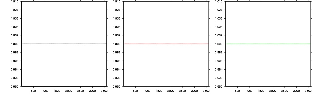
Figure 1 : The stability of external, slightly
internal and internal RH modes as a function of zonal horizontal wavelength
given in km. Meridional horizontal wavelength was fixed to 3600 km. The modes
are stable for the whole horizontal spectrum.
The relative phase-speed error is shown in Figure 2. Solid
curve represents the predictor and dashed curve the corrector. The external,
slightly internal and internal modes are plotted as the left, middle and the
right plot. The result is opposite to what could have been naively expected.
The PC scheme accelerates the RH modes. However, the acceleration is very
small about 0.1 %. The horizontal wavelength of accelerated modes depends on
the vertical mode. The magnitude of acceleration is negligible comparing to
the effects caused by other, mainly physical processes.
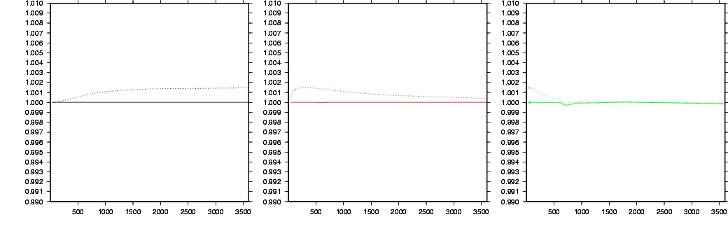
Figure 2 : The relative phase speed error of
external, slightly internal and internal RH modes as a function of zonal
horizontal wavelength given in km. Meridional horizontal wavelength was fixed
to 3600 km. The PC scheme slightly accelerates the modes. The magnitude of
acceleration is about 0.1 % and it is too small to have any practical impact
on mesoscale model simulations.
Lothar storm case study
To test the accuracy of the model for synoptic scales the
Lothar storm case was chosen. It is the first of the two storms from December
1999 that passed over Europe during Christmas. The meso-cyclone formed over
Atlantic Ocean and it moved rapidly towards Europe. During the 26th of
December 1999 the storm hit France, Germany, Switzerland and Italy and caused
severe damages. Operational forecast of the global model ARPEGE provided
reasonable guidance for Lothar storm. When ALADIN is coupled with ARPEGE
prediction using quadratic coupling or 3 hour frequency coupling, the
prediction of Lothar storm is sufficiently accurate to be considered
successful in the view of current LAM performance. In Figure 3, we can see the
26th December 1999 analysis of ARPEGE at 12, 18 and 24 UTC.
The Lothar storm is possible to predict using the dry
adiabatic model version. However, such prediction is not possible to verify
against the model analysis. Therefore we used the diabatic version of model
ALADIN. We run the prediction using initial condition from 12 UTC on the 25th
of December 1999. The reference run was obtained with hydrostatic model
version using the two-time-level SI SL scheme with LSETTLS
extrapolation (Figure 4). The integration domain was the
ALADIN/LACE domain, the horizontal mesh size is 12.2 km and D
t =600 s. The position of the cyclone is shifted slightly to the
east and is 1 hPa shallower (972 hPa in the centre) than in the analysis (left
plot in Figure 3).
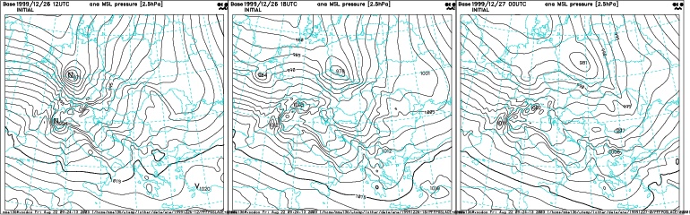
Figure 3 : The 3d-var analysis of model ARPEGE,
of the Lothar storm case from the 26th of December 1999. The mean-sea-level
pressure is plotted with contour interval 2.5 hPa. The storm moved eastward
over France, Germany and finally during the 27th of December 1999 it weakened
over southwest Poland.
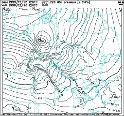
Figure 4 : The 24 h reference prediction of
Lothar storm from 25th of December 1999 12 UTC. The prediction obtained with
hydrostatic model version with 2TL SI SL LSETTLS scheme. The results obtained
with the 2TL SI SL non-extrapolating scheme
To assess the impact of ICI scheme itself, we integrated the
Lothar case using the two time-level non-extrapolating ICI scheme with
hydrostatic model version. The method of extrapolation used to compute
nonlinear residuals and the wind for trajectories was changed. The first order
accuracy algorithm in time was used during predictor, while LSETTLS approach
is second order accuracy. The second order accuracy is restored during
subsequent iterations.
The physics was called once per time step, during predictor.
The physical tendencies were considered to be valid in departure point of SL
trajectories at time instant t.
In the left column of Figure 5, the 24 h prediction is showed
computed with ICI scheme using different number of iterations (equivalent to
n=0 and 1 as defined in 3
]). The top left plot is calculated using two-time-level SI
non-extrapolating scheme described by 4
]. As it was mentioned already, it is a first order accuracy scheme, but
the obtained results are reasonable in the case of Lothar storm. The cyclone
is well positioned and the minimum mean-sea-level pressure (MSLP) is
underestimated by 1 hPa comparing to analysis. Further iterations of the SI
solver using ICI scheme did not bring any significant change in storm
prediction. The differences between the SI non-extrapolating scheme and the PC
scheme predictions are showed on top right plot of Figure 5 The maximum
difference is 2.1 hPa. The PC scheme prediction itself is displayed in the
bottom left plot and the differences gained by further iteration of ICI scheme
are showed on the bottom right plot. It is apparent that the scheme is
converging since the differences between successive iterations of the ICI
scheme converge towards zero.
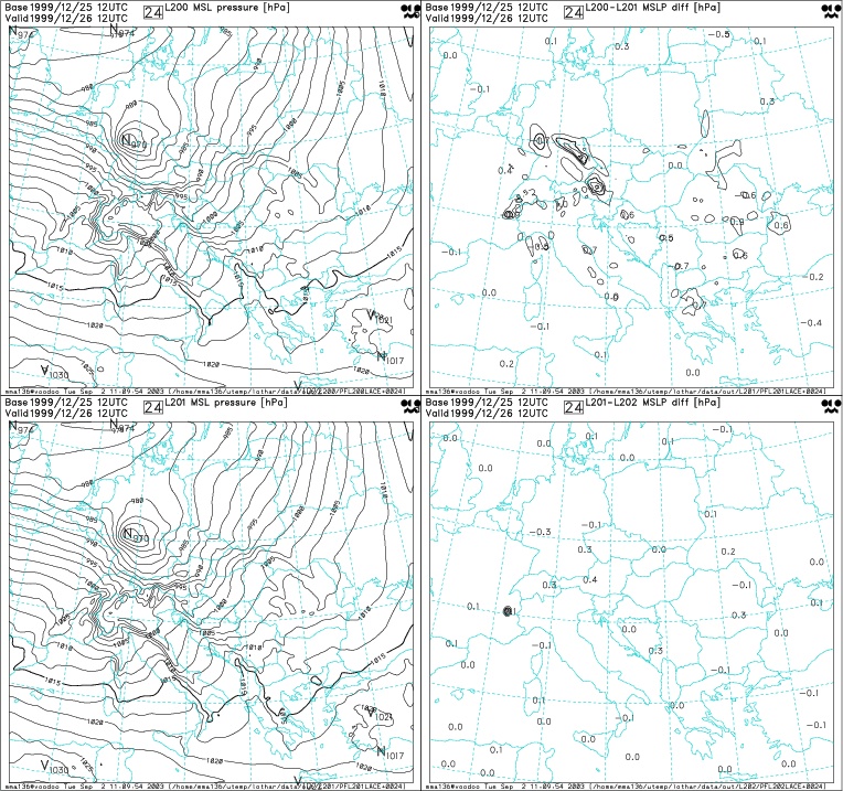
Figure 5 : The 24 h prediction from 25th of
December 1999 12 UTC obtained with the 2TL ICI SL non-extrapolating scheme
with n=0 (top left plot) and n=1 (bottom left plot). The
differences between the runs with different number of iterations of ICI scheme
are plotted in the right column. The differences between the SI scheme and the
PC scheme runs are on top right plot, and the differences between the PC
scheme and ICI scheme with n=2 are on the bottom right plot.
We have integrated the Lothar case using the non-hydrostatic
model version as well. We used the prognostic variable d4 (namelist
variable NVDVAR=4) and we
set the SI acoustic temperature to 50K and keep the value of SI gravity
temperature 350 K (namelist variables SITRA
=50 K and SITR
=350 K, for detailed explanation see Bénard, 2004). We used the
2TL ICI non-extrapolating scheme with SL advection. The results are showed on
Figure 6. Comparing to the equivalent hydrostatic run, there is a further
underestimation of the minimum MSLP by 1 hPa, but this difference disappears
after the first iteration of ICI scheme. The results obtained with the
non-hydrostatic model version are almost identical to the hydrostatic results.
This proves that the tested scheme applied on ALADIN's non-hydrostatic
dynamics efficiently stabilises all the possible sources of instabilities for
the "hydrostatic" time step length (orographically induced waves,
SHB temperature and pressure instabilities), while keeping the quality of the
simulation of the large scales as in the hydrostatic model. We can deduce from
Figure 6, that the PC scheme is fully sufficient to integrate the model for
resolution around 10 km, because there is no significant change in the results
when using two or more iterations of the SI solver.
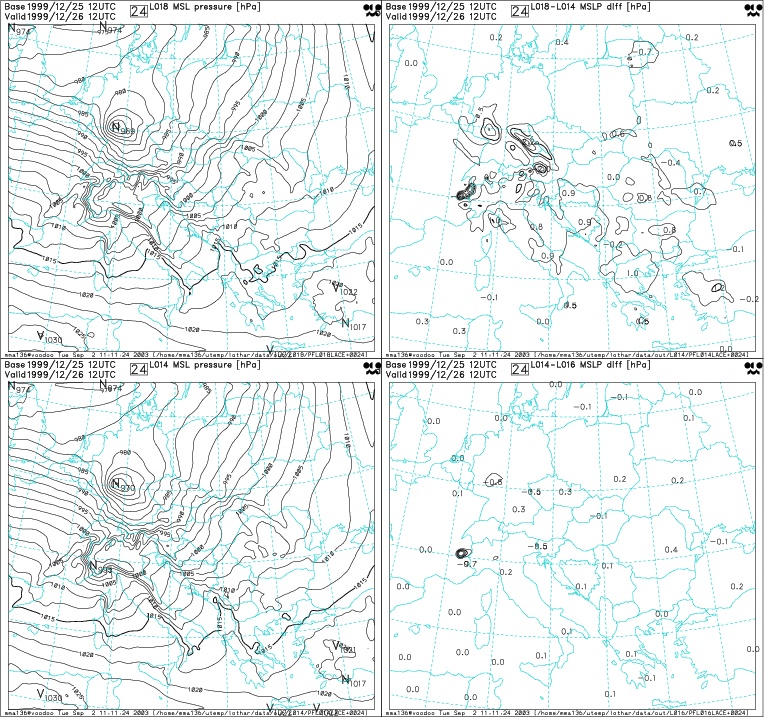
Figure 6 : The same as on Figure 5, but obtained with the
non-hydrostatic version of ALADIN.
The aim of this study was to show that the 2TL ICI scheme
doesn't deteriorate results obtained with the standard SI scheme when applied
to a synoptic scale case. The linear analysis indicated that the RH modes are
slightly accelerated by two-time-level PC scheme. The frequencies of the RH
modes are 0.1 % greater than their analytical value. However, there are still
nonlinear residuals not included in the analysis and a case study with the
full nonlinear model has to be carried out to draw a final conclusions. We
showed that the acceleration and remaining nonlinear residuals had no impact
on accuracy of short-range diabatic model integration.
The results obtained with 2TL ICI SL non-extrapolating scheme
with either hydrostatic or non-hydrostatic version are almost equivalent to
the reference results from the hydrostatic model integrated using the 2TL SI
SL LSETTLS scheme at the 10 km scale. This confirmed that the partially
implicit treatment of slow modes in ICI scheme doesn't deteriorate them.
The simulations using the non-hydrostatic model version
further proved that the methods used to stabilise acoustic modes and the
orographically induced instabilities are neutral to slow modes. The Lothar
case study proved that for resolutions around 10 km the 2TL SL PC
non-extrapolating scheme without additional filtering is sufficient to
integrate NH model ALADIN formulated with the prognostic variables d
4, P and q. No significant improvement can be gained by
additional iterations of the SI solver.
Bibliography
1] Bénard, P., 2003 : Stability of
semi-implicit and iterative centred-implicit time discretization for various
equations systems used in NWP, to be published in MWR.
2] Bénard, P., 2004 : On the use of
a wider class of linear systems for the design of constant-coefficients
semi-implicit time-schemes in NWP, to be published in MWR.
3] Laprise, R., 1992: The Euler equations
of motions with hydrostatic pressure as an independent variable. Mon. Wea.
Rev ., 99, 32-36.
4Lindzen, R.D., 1967 : Planetary waves on
beta-planes. Mon. Wea. Rev., 95, 441-451.
5] Temperton, C., 1997: Treatment of the
Coriolis terms in semi-Lagrangian spectral models, In: Numerical methods in
atmospheric and oceanic modeling. The André J. Robert Memorial
Volume . NRC Research Press.
non-hydrostatic dynamics stability of
Rossby-Haurwitz modes.
Theoretical and practical aspects.
Introduction
The class of schemes that are iterative approximations to fully implicit schemes applied on the Euler-equations (EE) system was studied in Bénard (2003). Any scheme of that kind is referred to as Iterative Centred Implicit (ICI) scheme in further text. The Semi-implicit (SI) scheme and Predictor/Corrector (PC) scheme are special cases of ICI scheme, with one respectively two solutions of the semi-implicit solver.
The EE system permits the gravity, acoustic and Rossby-Haurwitz (RH) modes. The stability analysis of the gravity and acoustic modes has been performed in Bénard, (2003) with EE system cast in hydrostatic pressure based s vertical coordinate of Laprise, (1992). The stability of small amplitude oscillations was studied in an isothermal atmosphere with temperature T0 over flat terrain. It was found that the gravity and acoustic modes are conditionally stable even in the limit of infinite time step, when an appropriate set of prognostic variables is used. The two-time-level predictor/corrector scheme is stable, if T 0 and the SI reference temperature T* satisfy condition : 1/2 T* < T0 < 2 T*. Nevertheless, the classical two-time-level (2TL) SI scheme is stable only if the background and the SI reference temperatures are equal, and the PC scheme becomes compulsory for realistic simulations which are naturally non-isothermal.
The Rossby-Haurwitz (RH) modes are usually treated explicitly in the models with the SI time stepping. With introduction of the two-time-level schemes with semi-Lagrangian (SL) advection treatment, the Coriolis force terms are treated semi-implicitly in some models (Temperton, 1997). The RH modes are partially implicit in a PC scheme as well. It is known that the implicit treatment of a mode slows it down. This is an acceptable behaviour for the modes that are not of meteorological interest (gravity modes in large scale hydrostatic models, or acoustic modes in non-hydrostatic models). However, RH modes are the main synoptic scale signals and their accurate representation is a necessary condition to consider the scheme to be applicable in a local area model.
Here, we analyse the free RH modes on a middle latitude b plane in the framework described previously. We are interested in the stability and accuracy properties of the RH modes in the limit of long time steps under the conditions for which the gravity and acoustic modes are stable.
The linear system with RH modes
The analysed linearized system of prognostic equation around isothermal, resting and isothermally balanced state yields:
(1)
We have used the formulation with prognostic variables q=ln(ps ), d=-gp/pRT×s× ¶ w/¶s, and P=(p- p )/p . f 0 is the Coriolis parameter on a reference latitude and b is the South-North horizontal derivative of the Coriolis parameter on that reference latitude. This approximation is sufficient to describe the behaviour of RH modes on a limited size middle-latitude domain (Lindzen, 1967). The system is further referred to as A and is formulated using divergence and vorticity as prognostic variables (D resp. x). We consider the tangent plane, therefore a local Cartesian horizontal coordinate system (x,y) can be introduced and the arrays can be decomposed horizontally into bi-Fourier series. In such a framework, the horizontal wind components can be expressed in the terms of divergence and vorticity as :
(2)
(k, s) are the horizontal wavenumbers defined along axes on horizontal plane.
To obtain, the SI linear system B, used in this study, we set f0=0 and b =0, and substitute T0 by the SI reference temperature T* in the system 1 ].
The two-time level non-extrapolating ICI scheme
We analyse the stability and accuracy properties of the two-time-level non-extrapolating ICI scheme. The general ICI scheme written in vector formalism is :
(3)
with state vector X =(D, d, P , q, T, x). The n index denotes the order of iteration (nÎ (1,...,NSITER ; n=0 SI scheme, n=1 PC scheme). When the process converges the last term on the rhs will converge to zero. The state at the beginning X[t+Dt(0)] is unknown and 3 ] cannot be used to figure it out. The non-extrapolating two-time-level SI scheme is used to calculate it :
(4)
and therefore the particular ICI scheme is referred to as non-extrapolating ICI scheme.
The stability and phase speed error of RH modes in the two-time level non-extrapolating ICI scheme
Eigenfunctions of the system on the tangent plane are expressed in the form :
(5)
with n being the dimensionless vertical wavenumber. The associated vertical wavelength for a given n in an isothermal atmosphere is lz =2p/n H.
Assuming that the amplitude of the mode is time dependent and
:
, we can apply the
classical Von-Neumann analysis of stability and look for complex amplification
factors l . The stability is defined by the
magnitude of l and the relative phase speed
error rp can be computed as rp
=arg( l) /w
aD
t . The analytical frequency w
a is computed from the dispersion
relation of the system 1
].
The stability was computed for the horizontal spectrum of continental size domain (the zonal horizontal wavelength varies from 36 km to 3600 km). The meridional wavelength was fixed to 3600 km. The time step length used in analysis was 600 s. It is the settings of the case study in the following section.
The temperature of the isothermal atmosphere is T 0 = 300 K (vertical height scale H = 8.8 km). The SI scheme is determined by the reference temperature T*= 300 K and the acoustic reference temperature T a* = 50 K (for detailed explanation see Bénard, 2004).
We analyse three vertical modes to assess the behaviour of the RH modes in the whole spectrum. The mode with n =0, that represents the external mode of the model with top in infinity. To sample whole spectra we further choose the modes with the vertical wavelengths 10 km and 2 km (n=5.5 and n=27.5) . They are referred to as "slightly internal" and "internal" mode in further text.
The stability of predictor and corrector of the two-time-level PC scheme is shown in Figure 1. The dependence of stability on the horizontal wavelength (given in km) is shown. The modes are stable for all horizontal scales (from 36 km to 3600 km).
Figure 1 : The stability of external, slightly internal and internal RH modes as a function of zonal horizontal wavelength given in km. Meridional horizontal wavelength was fixed to 3600 km. The modes are stable for the whole horizontal spectrum.
The relative phase-speed error is shown in Figure 2. Solid curve represents the predictor and dashed curve the corrector. The external, slightly internal and internal modes are plotted as the left, middle and the right plot. The result is opposite to what could have been naively expected. The PC scheme accelerates the RH modes. However, the acceleration is very small about 0.1 %. The horizontal wavelength of accelerated modes depends on the vertical mode. The magnitude of acceleration is negligible comparing to the effects caused by other, mainly physical processes.
Figure 2 : The relative phase speed error of external, slightly internal and internal RH modes as a function of zonal horizontal wavelength given in km. Meridional horizontal wavelength was fixed to 3600 km. The PC scheme slightly accelerates the modes. The magnitude of acceleration is about 0.1 % and it is too small to have any practical impact on mesoscale model simulations.
Lothar storm case study
To test the accuracy of the model for synoptic scales the Lothar storm case was chosen. It is the first of the two storms from December 1999 that passed over Europe during Christmas. The meso-cyclone formed over Atlantic Ocean and it moved rapidly towards Europe. During the 26th of December 1999 the storm hit France, Germany, Switzerland and Italy and caused severe damages. Operational forecast of the global model ARPEGE provided reasonable guidance for Lothar storm. When ALADIN is coupled with ARPEGE prediction using quadratic coupling or 3 hour frequency coupling, the prediction of Lothar storm is sufficiently accurate to be considered successful in the view of current LAM performance. In Figure 3, we can see the 26th December 1999 analysis of ARPEGE at 12, 18 and 24 UTC.
The Lothar storm is possible to predict using the dry adiabatic model version. However, such prediction is not possible to verify against the model analysis. Therefore we used the diabatic version of model ALADIN. We run the prediction using initial condition from 12 UTC on the 25th of December 1999. The reference run was obtained with hydrostatic model version using the two-time-level SI SL scheme with LSETTLS extrapolation (Figure 4). The integration domain was the ALADIN/LACE domain, the horizontal mesh size is 12.2 km and D t =600 s. The position of the cyclone is shifted slightly to the east and is 1 hPa shallower (972 hPa in the centre) than in the analysis (left plot in Figure 3).
Figure 3 : The 3d-var analysis of model ARPEGE, of the Lothar storm case from the 26th of December 1999. The mean-sea-level pressure is plotted with contour interval 2.5 hPa. The storm moved eastward over France, Germany and finally during the 27th of December 1999 it weakened over southwest Poland.
Figure 4 : The 24 h reference prediction of Lothar storm from 25th of December 1999 12 UTC. The prediction obtained with hydrostatic model version with 2TL SI SL LSETTLS scheme. The results obtained with the 2TL SI SL non-extrapolating scheme
To assess the impact of ICI scheme itself, we integrated the Lothar case using the two time-level non-extrapolating ICI scheme with hydrostatic model version. The method of extrapolation used to compute nonlinear residuals and the wind for trajectories was changed. The first order accuracy algorithm in time was used during predictor, while LSETTLS approach is second order accuracy. The second order accuracy is restored during subsequent iterations.
The physics was called once per time step, during predictor. The physical tendencies were considered to be valid in departure point of SL trajectories at time instant t.
In the left column of Figure 5, the 24 h prediction is showed computed with ICI scheme using different number of iterations (equivalent to n=0 and 1 as defined in 3 ]). The top left plot is calculated using two-time-level SI non-extrapolating scheme described by 4 ]. As it was mentioned already, it is a first order accuracy scheme, but the obtained results are reasonable in the case of Lothar storm. The cyclone is well positioned and the minimum mean-sea-level pressure (MSLP) is underestimated by 1 hPa comparing to analysis. Further iterations of the SI solver using ICI scheme did not bring any significant change in storm prediction. The differences between the SI non-extrapolating scheme and the PC scheme predictions are showed on top right plot of Figure 5 The maximum difference is 2.1 hPa. The PC scheme prediction itself is displayed in the bottom left plot and the differences gained by further iteration of ICI scheme are showed on the bottom right plot. It is apparent that the scheme is converging since the differences between successive iterations of the ICI scheme converge towards zero.
Figure 5 : The 24 h prediction from 25th of December 1999 12 UTC obtained with the 2TL ICI SL non-extrapolating scheme with n=0 (top left plot) and n=1 (bottom left plot). The differences between the runs with different number of iterations of ICI scheme are plotted in the right column. The differences between the SI scheme and the PC scheme runs are on top right plot, and the differences between the PC scheme and ICI scheme with n=2 are on the bottom right plot.
We have integrated the Lothar case using the non-hydrostatic model version as well. We used the prognostic variable d4 (namelist variable NVDVAR=4) and we set the SI acoustic temperature to 50K and keep the value of SI gravity temperature 350 K (namelist variables SITRA =50 K and SITR =350 K, for detailed explanation see Bénard, 2004). We used the 2TL ICI non-extrapolating scheme with SL advection. The results are showed on Figure 6. Comparing to the equivalent hydrostatic run, there is a further underestimation of the minimum MSLP by 1 hPa, but this difference disappears after the first iteration of ICI scheme. The results obtained with the non-hydrostatic model version are almost identical to the hydrostatic results. This proves that the tested scheme applied on ALADIN's non-hydrostatic dynamics efficiently stabilises all the possible sources of instabilities for the "hydrostatic" time step length (orographically induced waves, SHB temperature and pressure instabilities), while keeping the quality of the simulation of the large scales as in the hydrostatic model. We can deduce from Figure 6, that the PC scheme is fully sufficient to integrate the model for resolution around 10 km, because there is no significant change in the results when using two or more iterations of the SI solver.
Figure 6 : The same as on Figure 5, but obtained with the non-hydrostatic version of ALADIN.
The aim of this study was to show that the 2TL ICI scheme doesn't deteriorate results obtained with the standard SI scheme when applied to a synoptic scale case. The linear analysis indicated that the RH modes are slightly accelerated by two-time-level PC scheme. The frequencies of the RH modes are 0.1 % greater than their analytical value. However, there are still nonlinear residuals not included in the analysis and a case study with the full nonlinear model has to be carried out to draw a final conclusions. We showed that the acceleration and remaining nonlinear residuals had no impact on accuracy of short-range diabatic model integration.
The results obtained with 2TL ICI SL non-extrapolating scheme with either hydrostatic or non-hydrostatic version are almost equivalent to the reference results from the hydrostatic model integrated using the 2TL SI SL LSETTLS scheme at the 10 km scale. This confirmed that the partially implicit treatment of slow modes in ICI scheme doesn't deteriorate them.
The simulations using the non-hydrostatic model version further proved that the methods used to stabilise acoustic modes and the orographically induced instabilities are neutral to slow modes. The Lothar case study proved that for resolutions around 10 km the 2TL SL PC non-extrapolating scheme without additional filtering is sufficient to integrate NH model ALADIN formulated with the prognostic variables d 4, P and q. No significant improvement can be gained by additional iterations of the SI solver.
Bibliography
1] Bénard, P., 2003 : Stability of semi-implicit and iterative centred-implicit time discretization for various equations systems used in NWP, to be published in MWR.
2] Bénard, P., 2004 : On the use of a wider class of linear systems for the design of constant-coefficients semi-implicit time-schemes in NWP, to be published in MWR.
3] Laprise, R., 1992: The Euler equations of motions with hydrostatic pressure as an independent variable. Mon. Wea. Rev ., 99, 32-36.
4Lindzen, R.D., 1967 : Planetary waves on beta-planes. Mon. Wea. Rev., 95, 441-451.
5] Temperton, C., 1997: Treatment of the Coriolis terms in semi-Lagrangian spectral models, In: Numerical methods in atmospheric and oceanic modeling. The André J. Robert Memorial Volume . NRC Research Press.