Application of the predictor-corrector method to non-hydrostatic dynamics

Introduction

The main event during reported period was the implementation of the predictor-corrector (PC) scheme into the main version of the ALADIN model (version AL25T1). The cleaning, optimization and debugging of PC scheme has been done. However only the two-time-level (2-TL) case has been coded up to now. We concentrated on idealized tests in order to validate the PC scheme against results from linear stability analyses. We implemented also an option with a non-isothermal semi-implicit background. The objective is to stabilise the PC scheme after the first corrector step for non-isothermal nonlinear flow regimes.

Implementation of PC scheme in ALADIN

The following formulations of the PC scheme have been implemented (written here without time-decentering although the decentering option has been implemented as well, L refering to the linear part and R to the nonlinear residual) :

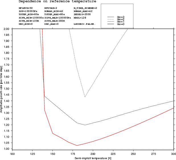
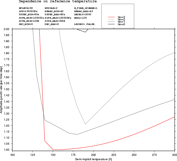
The non-extrapolating PC scheme was found to be more stable in linear analyses of stability (see Figure 1). It is a true 2-TL scheme without numerical modes (i.e. a non-oscillatory scheme) and is less expensive concerning memory.

Figure 1. Growth-rate per time-steps of the most unstable mode, for extrapolating (left) and non-extrapolating (right) schemes and the same atmospheric conditions, as a function of the semi-implicit temperature. (black dotted line : after the first corrector step, black solid line : after the second one, red solid line : after the third one).

Choice of Prognostic Variables

It has been found that the stability of the semi-implicit non-hydrostatic model significantly depends on the choice of the additional non-hydrostatic prognostic variables. The following non-hydrostatic prognostic variables have been chosen :

The pseudo vertical divergence d3 is equivalent to vertical velocity w, while P is equivalent to true pressure p. The choice of d3 ensures the stability, in sigma or eta coordinates, for linear flow regimes. The choice of P is important when eta coordinate is used in the vertical. The model is slightly more unstable after a first corrector step according to linear analyses of stability. With this variable, it can be integrated using semi-implicit time-stepping (predictor only) for linear flow regimes. This is not valid for the old prognostic variables.

All the results presented in this document were obtained using this choice for prognostic variables.

2D vertical plane tests

We found that the solution strongly depends on the choice of temperature for the isothermal semi-implicit background.

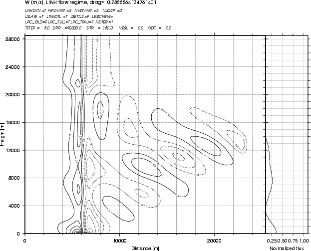
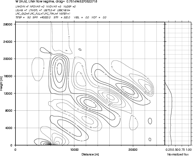
The best choices from the points of view of stability and accuracy may not be the same. On the figures below, linear non-hydrostatic flow regime tests (h coordinate, non-isothermal initial state with 220K at the surface and a vertical profile with constant Brunt-Vaisala frequency 0.01 s ^-1 ) are presented, where the only difference is the choice of semi-implicit temperature (SITR) : 180 K on the left plot and 300 K on the right plot.

There is an artificial chimney present right above the mountain when the lower temperature is used. As it increases, the chimney disappears, above approximately 270 K, the normalized momentum flux gets more realistic, but model becomes more unstable. The best choice for stability in this case would be approximately 260 K. That is the value we have chosen for the next tests.

From linear to nonlinear flow regime

We tested the stability properties of the PC scheme when going from linear flow regimes (where linear analyses of stability are valid) to nonlinear ones. Results are summarised in the following tables. CFL is the well-known Courant-Friedrich-Levy dimensionless number, calculated as for Eulerian time-stepping. Nonlinearity is characterised by a dimensionless number : NH/V, where N is the Brunt-Vaisala frequency of the background (initial) state, H the height of the Agnesi-shape obstacle and V is the wind speed of the background state. We chose N=0.01 s^-1 and V=10 ms ^-1. The linearity was thus controlled by the height of the obstacle.

We integrated the model using the PC scheme with no (NSITER=0), one (NSITER=1), two (NSITER=2) and three (NSITER=3) corrector steps. The length of integration (before model blew up) is multiplied by the wind speed and divided by the width of the obstacle to obtain a dimensionless variable and make comparison of integration lengths easier (as CFL is changing). The maximum dimensionless length of integration was 50, and the corresponding solution was considered to be already in a quasi-steady state.

We see that it is not possible to use a simple semi-implicit time-stepping when the initial temperature profile is non-isothermal with N=0.01 s ^-1. After a first corrector step, linear and quasi-linear flows are stabilised up to CFL=1.5. After a second one, all flows are stable for CFL around 1, but integrations with lower and higher CFL are unstable. We believe this is due to bad interactions between the "sponge" upper-boundary condition and dynamics. After a third corrector steps, all flows are stable up to CFL=2.

Isothermal versus non-isothermal semi-implicit background

To improve the convergence rate of PC scheme, we implemented a "non-isothermal semi-implicit background" option. We kept vertical operators as for the isothermal semi-implicit solver. According to analyses of stability, this choice should stabilise all linear regimes already after a simple semi-implicit time-step (NSITER=0). The results for NSITER=0 are shown in the tables below. Linear regimes are stabilised but there is almost no influence on more nonlinear regimes. The results after a first corrector step are not shown since there was almost no change, when comparing to results obtained with an isothermal semi-implicit solver (see the table for NSITER=1 in the previous paragraph).

This tests proved definitely that the instability in non-hydrostatic ALADIN dynamics is purely nonlinear.