Tendency coupling of the surface pressure

Tamás Szabó

1.  Introduction

The interpolation from the large scale model's orography to the nested model's one can cause imbalance in the surface pressure. If this happens in the coupling zone, the unbalanced pressure will be coupled. To decrease this harmful effect we implemented a tendency coupling scheme for the surface pressure. For more details about this topic see Szabó (2001).

2.  Coupling schemes in ALADIN

First it is worth comparing the old and the presently used coupling schemes.

2.1  The old t0 coupling scheme

This relaxation scheme was applied at the beginning of the gridpoint computations, so the derivatives also had to be modified, furthermore the gridpoint computations had to be done in the extension zone as well, otherwise biperiodicization would have been needed. The scheme was:

(1)

(2)

where a is the relaxation coefficient (Janisková 1994), Q is the model state vector, and the subscripts c and LS stand for coupled and large scale, respectively.

2.2  The presently used t1 coupling scheme

This scheme is applied after the gridpoint computations, just before the spectral transforms at the level of the SI equation, which is as follows:

(3)

where is the explicit guess, is the explicit part of the semi-implicit correction (see Bénard 1999), contains the whole RHS of the equation and L is the linear model. The gridpoint computations are not needed to be done in the extension zone, since the coupling scheme makes the fields biperiodic. The scheme is applied on intermediate quantities, not on the prognostic variables themselves (Radnóti 1995):

(4)

The coupled variables have to be similar quantities, thus the presence of the (I - bDt L) operator on the LHS of the SI equation shows that this operator has to be applied on before coupling in (4).

2.3  Comparison of the two schemes

The two above-mentioned coupling schemes are not equivalent:

(5)

where F is the Fourier transform, T and D are the truncation and the horizontal diffusion, respectively. A reason for this is that a is a horizontally changing variable, so it cannot be moved before the horizontal operators.

The t1 coupling changes the fields in the extension zone, so in the output the fields in the E zone differ from the large scale fields.

3.  The tendency coupling scheme

We start from the following equation:

(6)

After discretisation (6) yields the following for 2TL scheme:

(7)

Equation (7) differs from the flow relaxation scheme in the last two additional terms.

3.1  t1 version (not coded)

Originally it was planned to add the new terms to the t1 coupling scheme. In this case the scheme would be:

(8)

As it can be seen in (8), the (I - bDt L) operator should also be applied on and . The problem with (8) is that only large scale variables have meaningful values in the extension zone. A solution could be to neglect there, but it is not sure then, that the coupled fields will be continuous. The reason for this is that and can differ even at the edge of the C+I zone due to the t1 coupling. Thus e.g. the term in (8) should be biperiodicized, and although we only want to apply the scheme on the surface pressure, the biperiodicization would be costly in every time-step.

3.2  Splitted version (coded for 2TL with DM)

An other possibility is to place the additional terms to the beginning of the gridpoint calculations in the next time step. Thus this version consists of an original t1 coupling and a modification of the surface pressure and its derivatives at t0 level. In this case there is no need for the SI correction of the fields and the problem of the possible discontinuity disappears. The two steps are:

¾ t1 coupling:

(9)

¾ t0 level modification of the surface pressure in the next time step:

(10)

(11)

(12)

where Ps is the surface pressure and R is a multiplier aimed to stabilize the scheme, because experiments showed that it is unstable with R=1 . The reason for this is that due to the fact, that the t1 and t0 coupling are not equivalent, the separation of the tendency coupling scheme can distort the scheme, as if other a coefficients were used for the separated terms in the coupling scheme and thus the chance of an instability is also larger.

4.  Results

From the two aforementioned possibilities of the implementation of the tendency coupling scheme the splitted version was chosen to introduce into the ALADIN code by a new switch: LTENC. It was coded only for the 2TL scheme, so the experiments were only made on the hydrostatic model with SL2TL scheme. It was coded for both the quadratic and linear coupling, but there is a difference between them for technical reasons: for the quadratic coupling the tendency coupling is not applied at every NEFRCL step, only the original t1 coupling is done in these time steps. Although it breaks the ``continuity'' of the tendency coupling it did not seem to have any negative effect. For the linear coupling we put a new switch, LALLTC, that determines whether tendency coupling is applied in all steps or just t1 coupling in every NEFRCL steps. The multiplier R in (10-12) is called RTENC in the code and should be far enough below 1 to be stable, but close enough to 1 not to make a scheme, which differs from the original tendency coupling scheme very much.

4.1  2D experiments

The experiments were made on a linear hydrostatic flow over a 10m high Agnesi shaped obstacle. Most of them were started from and coupled with a perturbed surface pressure field by a 1hPa amplitude cosine wave, which had four wavelength in the C+I zone (first 180 points) and maximums at the edges of the C+I zone.

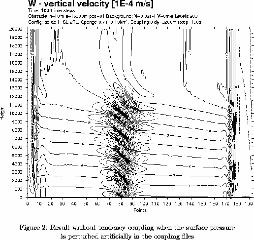
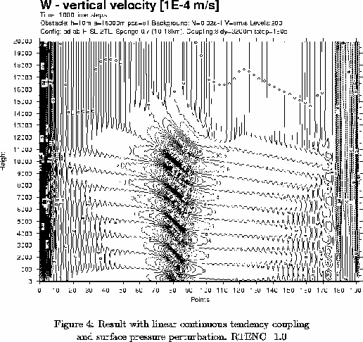
Figure 1 shows the vertical velocity when the surface pressure is perturbed. Now switching on the tendency coupling scheme (LTENC=. T.) with 10+1 identical LBC files, figure 2 shows the noisy results with a multiplier RTENC=1.0 for linear ``continuous'' tendency coupling (LALLTC=. T.).

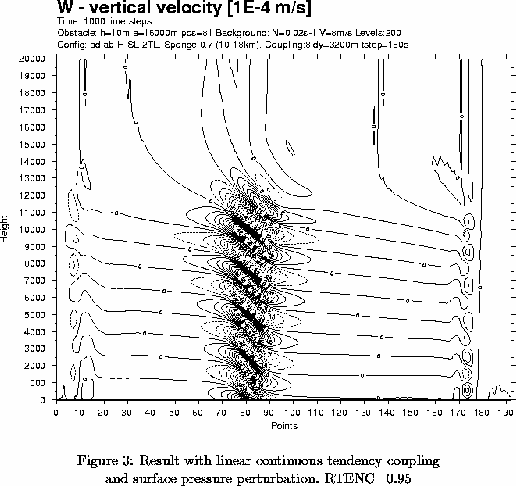
Decreasing RTENC to 0.95 the noise disappears (Figure 3) and the field looks better in the coupling zone. Increasing RTENC above 1.0 the model can blow up, e.g. with RTENC=1.1 it blows up after 89 steps.

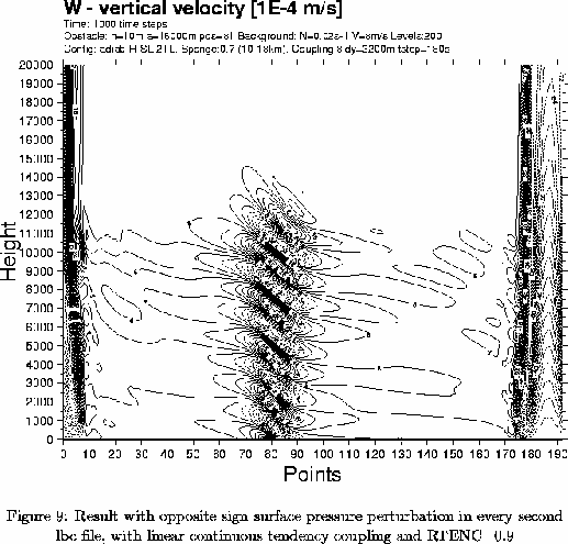
In the stable experiments the results with tendency coupling were better than those without it. A reason for getting good results was that the quality of the large scale tendency was better than that of the large scale field, i.e. the surface pressure perturbation was constant, so the large scale tendency was zero. An experiment was made to try a worse quality large scale tendency by using an opposite sign surface pressure perturbation in every second coupling file. The results were similarly bad for both the original t1 coupling (not shown) and the tendency coupling case with RTENC=0.9 (Figure 4). RTENC=0.95 gave noisy result in this experiment.

4.2  3D experiments

We ran the full model for only one case: the 1st of April 2001 on the LACE domain. For RTENC=1.0 the tendency coupling schemes seemed to be stable, at least I could not recognize any instability, and the verification results were sometimes better sometimes worse than that of the operational model. Although the previous case seemed to be stable we tried it with RTENC=0.9 to compare the accuracy. The verification results were similar, perhaps a little bit worse.

When RTENC=1.1 was set the model did not blow up, but the verification results were much worse. Of course one 3D experiment is only enough for a preliminary check, not for evaluation.

5.  Modifications in the code

The tendency coupling scheme was coded only for 2TL scheme with DM. It is not coded for LSPLIT and B level parallelization, neither for NEDFI=6. The modifications of AL13 subroutines can be found in Prague in the directory sx4:/home/mma/mma142/AL13_tc.

6.  Conclusion

The interpolation of the surface pressure from the large scale model's orography to the nested model's one can cause imbalance in the surface pressure field. This can result in the coupling of the unbalanced pressure. To decrease this harmful effect we applied a tendency coupling scheme for the surface pressure. It consists of a t1 coupling and a modification of the surface pressure and its derivatives at t0 level. This scheme proved to be unstable in 2D experiments probably due to the splitting of it, but a simple modification of the scheme made it stable. The results of the 2D experiments are better with tendency coupling, when the surface pressure is perturbed and has constant value in time in the LBC files. When the surface pressure perturbation changes sign in every next LBC file the results of the tendency coupling scheme are similarly bad as those of the original t1 coupling scheme. A 3D experiment shows that the quality of the forecast with the tendency coupling scheme is probably similar to that of the operational model. The tendency coupling scheme was coded for the 2TL scheme and DM, the newest version of the modified subroutines of AL13 can be found in Prague in the directory sx4:/home/mma/mma142/AL13_tc.

References

P. Bénard (1999), Scientific documentation for ALADIN NH model

M. Janisková (1994), Study of coupling problem

G. Radnóti (1995), Comments on ``A spectral limited-area formulation with time-dependent boundary conditions applied to the shallow-water equations'', MWR, Vol. 123, 3122-3123.

T. Szabó (2001), Tendency coupling of the surface pressure and related modifications in the code, Prague report

Figure 1: Result without tendency coupling when the surface pressure is perturbed artificially in the coupling files

Figure 2: Result with linear continuous tendency coupling and surface pressure perturbation. RTENC=1.0

Figure 3: Result with linear continuous tendency coupling and surface pressure perturbation. RTENC=0.95

Figure 4: Result with opposite sign surface pressure perturbation in every second LBC file, with linear continuous tendency coupling and RTENC=0.9

Home