An improved method to incorporate lateral boundary conditions in a spectral limited area model

Gábor Radnóti, January 2001

Introduction

This study was stimulated by the famous "Christmas storms" of 1999 (26 and 27 December). In these cases two very intensive, rapidly propagating meso-scale cyclones, that developed over the middle Atlantic, passed Western Europe. The forecast of these systems failed in most global models, partly because around the times of cyclo-genesis only one observation over the Atlantic indicated the existence of the systems and most of the data assimilation schemes have rejected these observations. However, the French global model ARPEGE kept them and the cyclones were "reconstructed" by the assimilation procedure. Therefore the ARPEGE forecast of the "Christmas storms" was reasonably good, although the size of the systems was at the limit of scales that can be resolved by the global model ARPEGE.

In such a case one would naturally expect that a higher resolution limited area model (LAM) coupled with this basically correct global forecast performs even better in describing such a small scale system. However, it was not the case for ALADIN and the reason was easy to find. The quality of a forecast by a LAM is to a large extent determined by the quality of the coupling forecast. In the given case, a LAM has no chance to forecast the storm if the cyclo-genesis is outside its domain and at the same time the coupling model fails to forecast it. In such a case there is no way that the LAM gets any information through the lateral boundary conditions (LBC) on the existence and on the entry of the system to its domain. Even if the coupling model forecasts the system the coupling scheme may fail to pass the information to the LAM and it was the case for ALADIN for these storms. Most operational LAMs, including ALADIN, use the Davies relaxation scheme for the LBC treatment. In this scheme the global model forces the LAM only at a "narrow" bend at the lateral boundaries of the LAM domain. The width of this zone is typically at the range of 100 km. Additionally, the forcing field is not directly the forecasted field of the coupling model for the given time, but a field obtained by temporal interpolation between two forecasts of the global model (the time interval of interpolation is typically 3 or 6 hours). If the method is a simple polynomial (linear or quadratic) interpolation it may happen, and it was exactly the situation in the case of this study, that the system has no trace on the coupling zone within the time interval of the passage because at the initial time (T0) the system is fully outside the LAM domain and at the next coupling time (T1=T0+3h or T1=T0+6h) the system has already left the coupling zone and it is fully inside the domain. Since the coupling model passes information to the LAM only by its fields over the coupling zone at discrete times, the LAM has the chance to learn the entry of a system to its domain only if it had any trace on these spatially and temporally reduced sub-fields.

The aim of this study is to investigate the possibility to change the temporal interpolation scheme and/or the coupling scheme to overcome the limitations described above. The fact that ALADIN is a spectral model using Fourier expansions in both horizontal directions offers promising solutions. On the one hand we can change the temporal interpolation scheme by interpolating phase angles and amplitudes rather than gridpoint values. In this case at the interpolation step the complete fields of the coupling model are used and not only their projection on the coupling zone. Thus in principle it is possible to retrieve the approximate location and depth of a wave-like system at any time of the interpolation interval. The price that one has to pay for this is that of performing inverse Fourier transforms on the coupling fields at each time-step after the spectral interpolation. Such a solution may partly or fully solve the problem described. However, it may be the case that even such an improved interpolation is not capable for retrieving the trace of a system on the coupling zone, or that the Davies scheme does not perfectly passes to the LAM the characteristics of a small scale system entering the domain. If it is the case, there is a possibility to modify the Davies scheme by introducing an additional spectral coupling step. A spectral coupling scheme can be built up on the exact analogy of Davies scheme. The difference is that the relaxation scheme is introduced in the spectral space: small wavenumbers take over the role of coupling zone while large wavenumbers represent the inner zone of the Davies scheme. This procedure provides a scale selection where "large scales" are dominated by the spectra of the coupling model and the LAM dominates only the small scales poorly, or not at all resolved by the forcing model. In such a scheme scales resolved by the coupling model are forced to the LAM no matter what the location of a system of the given scale is within the domain. Therefore the LAM surely captures any system resolved by the coupling model and not only at the time of passage through a narrow lateral zone. This is a tempting potential advantage of spectral coupling. However, one can easily see that spectral coupling itself can not take over the role of LBC treatment, since even the expression "lateral boundary" is meaningless in the case of spectral coupling, where there is no geographical selection. Consequently spectral coupling can not eliminate spurious wave reflection from lateral boundaries (or in the case of a spectral LAM spurious inward wave propagation through the lateral boundaries), that is one of the primary aims of using coupling schemes. Nevertheless, one may hope that a careful simultaneous use of Davies scheme and a "well-tuned”" spectral coupling can optimally combine the advantages of the two methods.

The following sections will discuss these possibilities with some spectral diagnostics and model tests on one of the "Christmas storm" cases.

Amplitude-phase-angle representation of ALADIN spectral fields to improve shape preserving properties of time-interpolation

The spectral representation of ALADIN fields is that coming from the subsequent one-dimensional FFTs (Fast Fourier Transform). As an example, when performing direct transformations, direct FFT is performed on each "latitude" and the resulting Fourier coefficients are transformed again by direct FFT along a "longitude". For a given zonal wavenumber the second transformation involves 2 FFTs, one performed for the real part and the other for the imaginary part. Therefore in the final result of the double FFTs a total wavenumber (j,k) j,k=0 can be described by 4 independent coefficients:

where rr means the real part of the second FFT on the real part of the first FFT, while ri ir and ii are the other three possible combinations. This representation is obviously not exactly the same as the coefficients in the two dimensional Fourier series:

(x, y being scaled into [0, 2p] ). However, it is easy to deduce the conversion relationships between the two representations. The result is:

When linear interpolation is performed between two fields the result is the same no matter if it is performed on the gridpoint values or on the spectral coefficients, and no matter which one of the above described two spectral representations is used (this is because both FFT and (1) (2) are linear in Q). Another possibility would be to perform the interpolation between amplitudes and phase-angles. The potential advantages and problems related to this will be discussed later. Now we want to see how one can obtain such a representation from the standard one. First let us consider the 1 dimensional case:

The amplitude phase angle representation means that a wave is described by _Aj sin ( jx + l_j ). This means that for a wavenumber j > 0 :

must hold, the left hand side being the cumulated contribution of wavenumber j in the 1 dimensional Fourier series :

.

Consequently :

The left hand side contains imaginary terms that must vanish. This leads to the complex conjugate relationship between positive and negative indices. Then we obtain :

Now let us consider the problem in two dimensions. Analogously to (3) the Fourier series contributes to a positive wavenumber pair j, k >0:

On the analogy of (3) the first two terms of (5) define a wave with amplitude and phase angle _Aj,k , l_j,k  and the second two terms another wave with amplitude and phase angle _Bj,k , m_j,k , and the result is a superimposition of the two plane waves:

Then the counterpart of (4) is :

and reversely :

For the set of (j,k) plane waves the total wavenumber direction is in the first quarter of the plane, while the set of (j,-k) pairs falls in the fourth quarter. It means that the total set of the waves spans the half-circle, as it can be expected:

If j=0 or k=0 (but not both are zero), then (5) contains only 2 terms and the problem reduces to the one dimensional case. Then the first two equations of (7) and (8) are sufficient. The missing pairs (-j,k) and (-j,-k) of (8) can be determined from the complex conjugate relationships. The combination of (1) and (7) provide the conversion formula in one direction and the combination of (2) and (8) in the opposite direction. Then the temporal interpolation between the spectral fields can be realized by a 3 step algorithm: for each wavenumber pair the two phase-angle amplitude pairs are computed, then the interpolation is performed between amplitudes and angles, finally the so obtained new amplitudes and phase angles are transformed back to obtain the new spectral coefficients.

The potential advantage of such a scheme can be illustrated on Fig. 1 in one dimension:

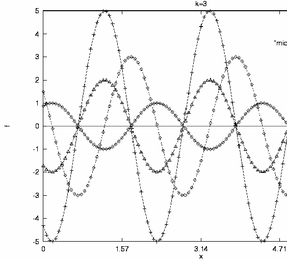
Figure 1 : A single wave (wavenumber=3) at initial, final time and at middle time obtained with different interpolations

We can see four waves with wavenumber 3. We defined a wave with a given amplitude and phase as an initial wave and another one with an increased amplitude and shifted phase as a final wave. Let us assume that we want to estimate the state of the evolving wave in the middle of the time interval. It is reasonable to assume that it is the amplitude and the phase of the wave that evolve linearly rather than the gridpoint values. The first assumption leads to the interpolated wave denoted by squares and the second leads to the curve denoted by triangles (and exactly this second curve would be obtained if spectral coefficients were interpolated). We can see that the two results differ significantly: The second choice results in a wave that is in phase very close to the final wave, while the first choice by definition results in a wave which is exactly in middle phase with middle amplitude. The reason for the "failure" of gridpoint interpolation is that the final wave is significantly stronger than the initial one. Consequently, the result of interpolation, as far as phase angle is concerned, is dominated by the final state. In reality one may think that the wave is deepening gradually and this is the most advantageous feature of phase angle/amplitude interpolation.

It is a little bit more interesting to see the same problem for a wave packet. Fig. 2 illustrates an initial wave packet and its future state.

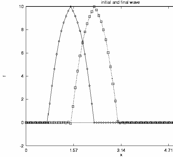
Figure 2 : A wave packet at initial and final time: phase speed is constant

For the sake of simplicity here we assumed a constant phase speed, which in this case is equal to the group velocity, and we also assumed time independent amplitudes for each wave component. Therefore the whole simple structure propagates in time without any deformation. Then we performed time interpolation to the middle time. Fig. 3 shows the result of linear interpolation for the middle time together with the initial state.

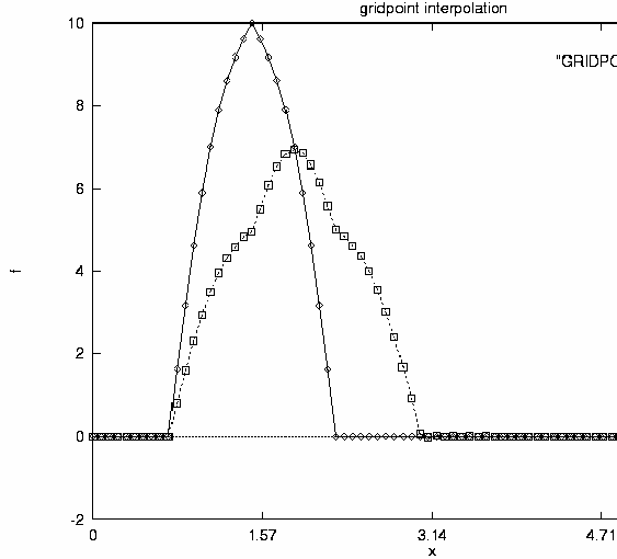
Figure 3 : Result of gridpoint interpolation and the initial wave packet

We see that the interpolation strongly modifies the shape of the wave packet. When we want to improve it by interpolating phase angles a serious aliasing problem occurs: Although the whole system propagated only by p /4, for a single wave of wavenumber k the shift in phase angle is kx p /4, that is already for relatively small wavenumbers bigger than 2x p. If the interpolation does not take into account this fact (phase angle of final state is converted into [0 , 2x p] and interpolation is in the shorter direction between the two phases) the result of phase angle interpolation is seen on Fig. 4, which is the worst among all.

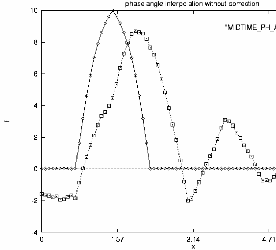
Figure 4 : Result of phase angle interpolation (modulo is neglected) and initial wave packet

However, if the modulo (number of 2p passages) is taken into account the result, as expected, is perfect (Fig. 5).

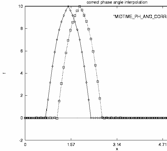
Figure 5 : Result of phase angle interpolation (modulo taken into account) and initial wave packet

To take the modulo exactly into account is not easy in the general case when the phase speed and the group velocity varies with the wavenumber and also with time, i.e. the temporal evolution is dispersive. It is a problem that has to be deeply analysed. In the NWP framework a first-order approach can be that for each wavenumber (in 2 dimensions for each wavenumber pair) the one time-step tendency of the corresponding phase angles provides an estimation for the total phase shift of the given time-interval. From this one can estimate the number of full periods of phase angle in that time interval to be added to the phase angle of the final state before doing the time interpolation. This can work well only if the phase speed of a given wavenumber pair does not strongly vary within the time interval. This can be true in most cases, but perhaps not in the most extreme situations, which are in the scope of our main interest in this study.

Let us assume that an intensive, relatively small scale system is rapidly approaching the domain of integration. It is reasonable to believe that the propagation speed of the system is strongly linked to the group velocities around the typical scale of the system. However at the initial time, when the phase speeds are estimated from the model tendencies, the given system has not yet reached the model domain therefore the extrapolation of these phase speeds to a time when the system is fully inside the domain might be misleading. With other words, the phase speeds may have a sharp change around the time when the system enters the domain. Another problem is that this method would assume that the phase speeds of the coupling model are the same as those of the coupled one, since the estimation is from the coupled model tendencies and it would be applied for the coupling fields.

The above described problems may be a major drawback of the proposed method. However, it is something to be carefully studied by a spectral analysis of model fields.

Another method can be also tested to estimate the modulo: although the phase speeds and group velocities vary with wavenumber, one can assume that it has some regularity that permits the persistence of wave packets. This may help to find the correct modulo: we may also assume that at the smallest wavenumbers the modulo is 0 or ±1 (the longest waves do not travel more than a full wavelength within a few hours). In one dimension we have the relationship :

-c (k) = ( l (k,T) + 2 n(k) p - l (k, 0) ) / kT (9)

where c is the phase speed, l is the phase angle, k is the wavenumber, n is the modulo within the time interval T of interpolation. We assume that for "small" wavenumbers n(k) = 0, 1 or -1, that one is chosen which results in the minimal | c(k) | (this means that the "shorter" phase direction is chosen between the initial and final phase angle). This estimation for small wavenumbers is reliable because here the denominator in (9) is relatively small, so changing the numerator by 2p would surely result in an unrealistically large phase speed. So we may assume that for k = 1, 2 we have a good estimation of c(1) and c(2). We continue on, apply (9) for the step by step increased wavenumbers keeping n(k) on its initial n(1) value as long as there is a sharp change in c(k) or rather in the group velocity c_g(k) = (k+1) c(k+1) - k c(k) . Then we eliminate this jump by increasing or decreasing n(k) by one. Algorithmically it means that from c(k) and c_g(k-1) we give an extrapolation for c(k+1), then we compute c(k+1) by using n(k+1)=n(k), n(k+1)=n(k) +1 and n(k+1)=n(k) -1 from (9) and that one of the three results is accepted which is closest to the extrapolated value. This is the one dimensional algorithm and it has to be generalized for 2 dimensions. The generalization may be done by the use of (6). Similar procedure can be introduced as described above. However, it is reasonable to simplify the problem in two dimensions and to use only the fundamental phase speed for computing the modulo for both waves represented in (6) : for the first wave in (6) one has :

(10)

where w_j,k is the angular velocity of the wavenumber pair (j,k).

From this we obtain :

w_j,k = ( l_j,k (T) + 2n_j,k p - l_j,k (0) ) / T (11)

The fundamental phase speed can be defined as :

where L_x and L_y are the domain sizes in x and y directions respectively. The algorithm for computing the modulo is then analogous to the one dimensional case :

· For wavenumber pairs (1,1), (1,2) and (2,1) we use n_j,k =0, ±1, and for each we select the one giving the minimal total phase-speeds

· We gradually increase j and k and extrapolate according to a first order Taylor expansion: c_j,k = c_j-1,k + c_j,k-1 - c_j-1,k-1

· We compute (12) using n_j,k = _nj-1,k =0, ±1, n_j,k = _nj,k-1 =0, ±1, and select that value of n_j,k which gives the closest result to the extrapolation

Preliminary tests of the method by spectral diagnostics

The first thing to test is the mathematical correctness of the phase-angle/amplitude representation introduced in the previous section. To do this we took one of the spectral fields (temperature of the lowest model level), applied equation (1) and (7) and computed temperatures for each gridpoint by :

where m,n are the gridpoint indices, M,N are the total number of gridpoints in x and y directions and JMAX and KMAX(j) are the maximum wavenumbers that are specified by the type of truncation, that is elliptic truncation in our case (the rest of notations is as before). We compared the so obtained temperatures with the ones obtained by the standard inverse Fourier transforms and the results were identical (maximum difference of the two gridpoint fields over the whole domain was of the order of 10 ^-13).

Before applying the method for the ALADIN system we wanted to see the impact of the improved interpolation method on an idealized case in a spectral shallow water model. This model uses exactly the same spectral representation of wind speed and geopotential as the ALADIN model. The model runs on fully periodic fields without coupling.

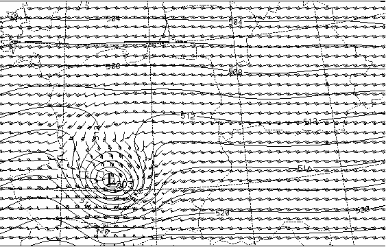
Figure 6.a : Zoom of a 12 hour integration of the spectral shallow water model

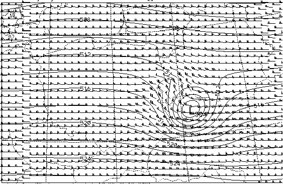
Figure 6.b : Zoom of a 18 hour integration of the spectral shallow water model

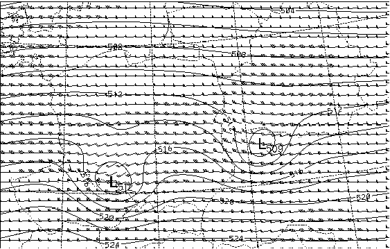
Figure 6.c : Zoom of gridpoint interpolation between 12h and 18h forecasts

As an initial state we have chosen a constant meridional geopotential gradient on the northern half domain and its opposite in the southern part to fulfil periodicity requirement. Then we put a perfectly circular cyclone over the northern part of the domain and we started from geostrophic balance. Then we used nonlinear normal mode initialization and integrated the model for 24 hours. To compare the two interpolation methods we have chosen the 12 and 18 hour forecasts. A zoom of the "active" area can be seen on Figure 6.a (12 hour forecast) and Figure 6.b (18 hour forecast). We can see that the cyclone is rapidly travelling eastward; in 6 hours it moved more than its characteristic size. Figure 6.c shows the result of linear gridpoint interpolation to middle of the time interval.

As we can see the interpolation is unsatisfactory: Instead of the propagation of the system we see that the initial cyclone is dying out and simultaneously the final cyclone is building up. If we assume that there is LAM embedded into this domain with a lateral boundary zone laying between the initial and final location of the cyclone, obviously this interpolation method will not pass any information on the entering cyclone.

Now let us see how the amplitude/phase angle interpolation performs for the very same case. At first we have visually analysed initial and final phase angle sets to get a first impression if the assumptions introduced in the previous section hold. We printed out initial and final phase angles of wavenumber pairs (j,j) (plane waves with NW-SE constant phase lines). The following table shows the results:

From the table we can see that phase speeds evolve quasi-regularly up to wavenumber pair (15,15) and it suggests that the algorithm proposed in the previous section might work well. It means that 2p passages can be safely identified for relatively small wavenumbers. At the second part of the spectrum it is not absolutely true, but we may hope that phase errors at those very small scales do not spoil the overall results because on the one hand the corresponding amplitudes are small and on the other hand phase error at a wave with very short wave length results only in a "few kilometre" shift of the given wave. After this "ad hoc" preliminary diagnosis the amplitude / phase angle interpolation was performed by the use of a slightly simplified version of the above proposed algorithm. The result can be seen on Figure 6.d .

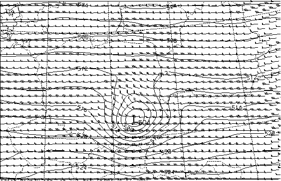
Figure 6.d : Zoom of amplitude / phase angle interpolation between 12h and 18h forecasts

We can see that the interpolation is much better than the gridpoint interpolation: the cyclone track is well represented without any artificial weakening, that was an undesirable feature of the gridpoint interpolation results.

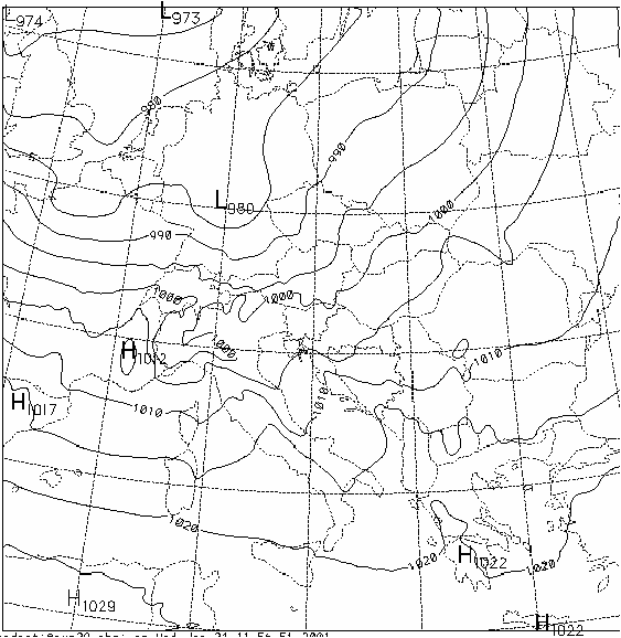
After this we repeated the tests for ALADIN with one of the Christmas storm cases. In this case, unfortunately, the phase angles did not indicate any regularity for non of the state vector components. We also tested one time-step tendencies of phase angles computed inside the model, but these neither indicated any persistence. Therefore we could try amplitude/phase angle interpolation only without unaliasing algorithm. The results of amplitude/phase angle and gridpoint interpolation were surprisingly similar (Figure 7.a-c).

The first two figures show how the mesoscale cyclone was rapidly moving, but the interpolation significantly smoothed it out and we can see the "bipole" structure, although not so strongly as in the gridpoint interpolation on the shallow water model results. It has to be mentioned that the interpolation was not directly performed on mean sea level pressure, but on the model state vector components and mean sea level pressure was obtained only afterwards by post-processing. It is very probable that the pure state vector components are not suitable for such a method, since its components do not clearly exhibit "propagating wave" structure. One has to investigate how the state vector should be transformed before the interpolation to take the benefit indicated by the shallow water experiments.

Parallelly we plan to investigate the possibility of combining standard coupling scheme with spectral coupling and the overall impact of amplitude-phase angle interpolation combined with Davies coupling.

Figure 7 : a. 18 hour mean sea level pressure forecast ; b. 24 hour mean sea level pressure forecast ; c. Result of amplitude phase angle interpolation

Home